As you sally forth into the land of structural equation modeling (SEM), you’ll come across terms like identification, and ideas like degrees of freedom (df) for a chi-square goodness of fit test. For many students, df is one of the more puzzling aspects of SEM. Sometimes it isn’t entirely clear where those degrees of freedom come from or why they have the values that they do. This was certainly a sticking point for me during my introduction to SEM, and can continue to be from time to time (in fact, part of why I’m writing this article is to solidify my own understanding — learning by teaching, as they say). Lacking an understanding of how degrees of freedom function in the context of SEM drove me mad during my introductory days. If you are facing a similar frustration now, this article might help. It’s not intended to be a complete solution to all your df woes. Honestly, degrees of freedom can be kind of a moving target sometimes – especially in more complex cases. However, I hope that this article at least provides you a better idea of the rudiments lying under the hood of SEM. Bear with me y’all.

The setup. I decided to build my example for this article for use in Mplus. I set up a mock 5-variable data file containing a correlation matrix. I’m assuming that I’m going to be working with a structural model with 3 exogenous (predictor) variables and 2 endogenous (outcome) variables.  I [very creatively] named them X1, X2, X3, Y1, and Y2, respectively.  Here’s what my data look like (yes this simple input matrix below is the entire data set. Don’t worry, Mplus is cool like that).

1.00
0.10  1.00
0.32  0.22  1.00
0.44  0.16  0.15  1.00
0.24  0.40  0.27  0.19  1.00

So now that we have the data, let’s learn a bit about model df.

Where do a model’s degrees of freedom come from, exactly? The easiest way to understand this is to examine the basic idea behind SEM. What SEM consists of is describing relationships among variables (frequently with the goal of figuring out what sorts of things explain variance in one or more endogenous (outcome) variables). To do this, SEM methods primarily involve analyzing variances and covariances among your variables. When you specify and analyze a structural model, you’re basically saying “Hey, program, here’s a layout of a group of variables. I think this layout best describes the ways in which these variables are related to each other. Now go check the data and see if I’m right (or more accurately, go see how right I am).”
(Didn’t even say please… How rude.)

When you hand the program a specification in this fashion, you’re telling the program to go ahead and solve the equations that are indicated by your model. This is where two parts of the system come into play – observations and parameters.

Observations. The easiest way to think about observations in the SEM context is to look at all of the variables you have in your system, and then stick them into a matrix (often a covariance or correlation matrix). If you have k variables, then you can put those variables into a k x k matrix. In my case, the matrix contains 5 variables, so k = 5. Here’s what they’d look like in a k x k (5×5) covariance matrix (Yes, I realize I swapped the traditional row x column labeling convention around. Whatever. I’m a rebel. Honestly, it makes no difference for illustrative purposes):You’ll notice that half[ish] of the matrix is empty. This is pretty standard for k x k matrices. Why? Simple — the upper triangular portion is an exact copy of the lower triangular portion. There’s no need to list both. More importantly, it’s precisely this fact that leads us to the next key aspect of figuring out observations in the SEM context. The number of observations is simply the number of unique elements in the matrix. All the covariance elements shown above are the unique elements in that matrix. When you have only a couple of variables, you can pretty easily count the number of observations by hand, but in larger systems (e.g., 17 variables with a few latent variables thrown in just to piss us off to high hell and back), you’ll lose track quickly. In either case, the fool-proof way to figure out the number of observations is to apply the good old lower-triangular formula to find the unique elements in a k x k matrix (it has two forms. use whichever one you prefer:

Number of observations =

So here, with a 5 x 5 matrix, we’ve got [ (5(5+1) ) / 2 ] unique observations. Doing the algebra yields:

[ (5(5+1) ) / 2 ] = ( 5(6) ) / 2 = 30/2 = 15 observations.

If you prefer the alternative formula you’d get:

[ (5² + 5) ] / 2 ] = (25 + 5) / 2 = 30/2 = 15 observations.

So there are a total of 15 observations available in this system for any kind of SEM to put to use. Counting them up by hand yields the same result. See? 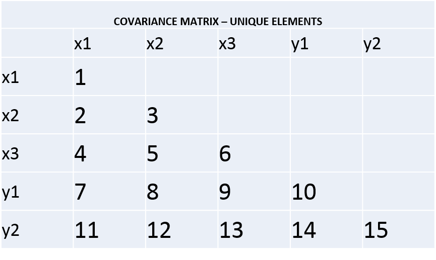Putting these 15 observations to use involves specifying parameters.

Parameters. A simple way to think about parameters is to see them as the equations that you ask the program to solve in order to estimate things for you. In order to solve the equations, the program will need to obtain and use information about the relationships among the variables in your model. This of course might lead you to wonder — “Where the hell does the information that parameters put to use actually come from?”  A fair question.

There are generally five key sources of information used for estimating parameters in any system of variables:

1. The variances of the exogenous (predictor) variables
2. The covariances among the exogenous (predictor) variables
3. The covariances between exogenous (predictor) and endogenous (outcome) variables. — these are often the prediction paths in the model, but not always.
4. The residual variances/error variances/unexplained variances/leftover variances/who-knows-what-explains-this-noise variances in the endogenous (outcome) variables,
5. Any covariances between these residual variances.

Sources 1, 2, and 3 are based directly on the covariance matrix elements we’ve seen already. Sources 4 and 5 are sort of ancillary components that are left over after the model has used information from sources 1, 2, and especially source 3 – however, they too are derived from the covariance matrix elements (namely the variances of endogenous outcome variables [#4], and covariances between these variables [#5]).

Now keep in mind — every time you specify a new, unique parameter in a SEM context, you use up at least one of your available degrees of freedom. It’s a sad fact of life, but hey, that’s what degrees of freedom are for. Asking the program to solve a brand new equation in your system of variables will require that the program uses up at least one of those sources of information that hasn’t been used yet (i.e., an observation is needed, so your df is reduced by 1). Notice that I keep saying “new” here. This is because you actually can specify parameters that don’t change your model’s chi-square value or df, if those parameters are defaults. We’ll see default parameters once we start testing models in a moment.

This point leads us to something I touched on very briefly at the opening of this article – model identification. I won’t get into identification in gruesome detail here, as it warrants its own article entirely, but one of the key things you need to keep in mind is simply this — a model can never have parameter specifications that require it to use more observations than there are observations available. If you attempt this, you end up with an underidentified model that has negative degrees of freedom, and your analysis program will usually explode when trying to estimate such a model.

It’s analogous to trying to follow the steps to put together a table when only 17 out of the 20 parts required are available. Your attempt to put together a structure that’s similar to what’s laid out in the manual can’t be completed because the manual is specifying more parts than there are parts to use. Same goes for model specification. The program ends up trying to estimate a structure that’s similar to what you’ve laid out in your model specification, but it doesn’t have enough parts (observations) available to construct an approximation (i.e., estimate the model) for you, so it just gives up and calls you an idiot (I’m fairly sure I’ve literally seen this language in my Mplus output. Mplus is a jerk sometimes). Long story short — don’t do this. Always be aware of how many degrees of freedom you actually have available when you want to test a model.

Now let’s see how parameters and observations come together to inform this process.

How observations and parameters determine degrees of freedom for a structural model. So now that we know where the observations and parameter information come from, we can begin to specify models. When we do this, we begin using up the degrees of freedom available. But wait… what are the degrees of freedom available when we first start? Glad you asked (I’m totally assuming you asked). Well, that, mis amigos, is determined by what we can call the empty model. The empty model is essentially the model where you specify that your variables exist in the matrix (i.e., they have variances) and you make no other claims about them at all. No means, no regression paths, no intercepts, no correlations or covariances, no correlated residuals, nada. They’re just sort of floating in SEM space. Conceptually speaking, it’s boring as all hell. Here’s what it looks like:

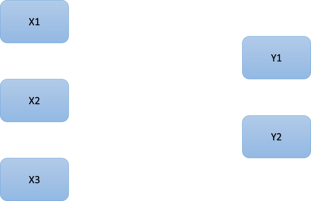Now this is probably the worst fitting model you can ever specify, because there is almost always at least SOME degree of association among a set of variables in a model (i.e., correlations are not EXACTLY zero in every case). But… do note that what we specified above requires observations from sources #1 and # 4 (from the list a few paragraphs ago) for estimating parameters. When you specify an empty model in Mplus, all of the variables in your system are treated as dependent variables. Because they’re treated as dependent variables that are unrelated to each other, the variance for each one is calculated by default, and that’s all you get.

Given that we are estimating variances for five variables, we now have five observations being used. So here’s where this leaves us:

Number of observations available for model estimation = 15
Number of observations used to estimate parameters = 5

The degrees of freedom for the test of model fit will equal the total number of available observations minus the number of observations that are actually used in order to estimate parameters. So in this case df = 15 – 5 = 10.

This leads us to another statistical property of these kinds of models. Because the number of observations used in an empty model is just equal to the number of variables in the system (k), the df for an empty model should always equal the number of observations minus the number of variables in the system. Expressed as a formula, we have:

df for empty model = [ ( k(k+1) ) / 2 ] – k

Expressed as an even simpler formula, just turn the + in the original lower triangular formula into a -, and we have:

df for empty model =  ( k(k-1) ) / 2

The answer is the same either way:

df for empty model = [ ( k(k+1) ) / 2 ] – k = [ ( 5(6) )/2 ] – 5 = [ 30/2 ] – 5 = 15 – 5 = 10.
—- or —-
df for empty model =  ( k(k-1) ) / 2 = ( 5(4) ) / 2 = 20/2 = 10.

To make things even clearer, we can zero in on the observations that have been used up by shading them in the original matrix, and seeing how it affects the df for this model. Chiggity-check it:

I went ahead and ran the empty model pictured above, assuming 350 participants provided my data. Mplus verifies what we’ve covered so far in its output (below). Note that “Number of free parameters” refers to all of the things that this model estimated freely (here it’s the 5 variances). It does NOT refer to the number of degrees of freedom in the model. It’s easy to confuse the two, so bear that in mind.

Number of Free Parameters                       5

Chi-Square Test of Model Fit

          Value                            223.777
          Degrees of Freedom                    10
          P-Value                           0.0000

Chi-Square Test of Model Fit for the Baseline Model

          Value                            223.777
          Degrees of Freedom                    10
          P-Value                           0.0000

Remember when I mentioned a bit earlier that you can specify default parameters and it doesn’t use up degrees of freedom? This empty model provides a good way to examine that. For example, if you explicitly specified an estimate of the variance of X1 as a parameter in this empty model, you’d end up with the exact same chi-square value and the df would remain the same — because this variance is estimated by default already.

Now you might be asking — “Why on Earth would anyone sit there specifying such a stupid and implausible model?” Fear not, weary traveler. This is what we might call a teachable moment. You see, the empty model has a nice property than informs the rest of the process of conducting SEM analysis. Running an empty model allows you to easily determine exactly how many estimable parameters of theoretical interest exist in your system of variables. Under normal conditions, the number of potentially estimable parameters of interest in your model is equal to the df for the empty model. In other words, any further models that you specify using these variables will start off with a certain number of estimable parameters, based on the df for an empty model. The df for an empty model tells you how many degrees of freedom you’ll be allowed to use when you start making specific, theory-driven claims about the relationships among the variables you have (e.g., correlated residuals, regression paths).

Alternatively, you can alter the degrees of freedom being used up by constraining certain parameters in your system of variables (e.g., telling the program that the correlation between X1 and X2 is equal to .85). This would turn a previously estimated parameter into a fixed parameter, and gain you back one sweet, juicy degree of freedom (though if your constraint is wildly inaccurate, you’ll compromise the fit of your model). Like model identification, this is a whole different topic altogether, so we’ll leave it at that for now (though we’ll see a bit of this later on).

Note that the “baseline model” in Mplus does not always correspond to the empty model. It is dependent on the things that are estimated by default, given your parameter specifications. For an empty model, it just so happens that the things that are estimated by default are identical to the things that are estimated due to your parameter specifications. This changes from model to model, as we’ll see a little later.

Now for a more realistic model. Now suppose we wanted to actually probe this system of variables in a meaningful way – we have a theory that X1 and X2 each predict Y1, while X1, X2, and X3 all predict Y2. We can lay that out like so:

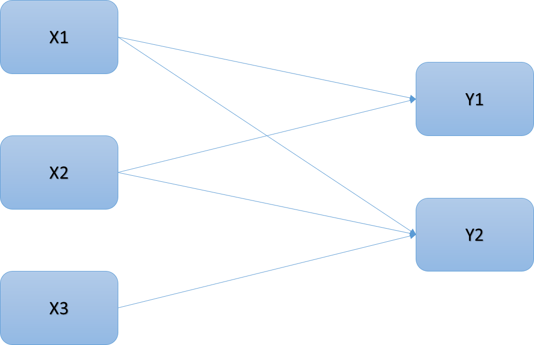
Here’s how I laid out my model in Mplus:
(Note — “ON” means “regressed on,” “WITH” means “covaries with/correlated with”)

Model:  y1 ON x1 x2;
        y2 ON x1 x2 x3;     

        y1 WITH y2;

This time we’ve specified 5 regression paths. Two of the variables in the system are treated as dependent variables (specifically the two endogenous outcome variables Y1 and Y2), so their variances are estimated freely by default (specifically, their residual variances). In addition, the covariance between these residuals is estimated by default. So this adds up to 2 residual variances + 1 residual covariance for the Y1 & Y2 outcome variables + the 5 regression paths, which brings our total number of freely estimated parameters to 8.

Recall that there were 15 total observations available in this system of variables. Referring back to the parameter info sources list from earlier, we can figure out that estimating this model would require the following observations:

1. 3 variances of the exogenous (predictor) variables.
2. 3 covariances among the exogenous (predictor) variables.
3. 5 covariances between exogenous predictors and endogenous outcomes.
4. 2 residual variances of endogenous outcomes.
5. 1 residual covariance between endogenous outcomes.

It will become even clearer why we need these observations once we see the model results a little later. Here’s where the list above leaves us:

Number of observations available = 15
Number of observations needed = 3+3+5+2+1 = 14.

So… df = 15 – 14 = 1.

There is only one parameter left for us to use in modeling this system of variables. It should be somewhat obvious what that parameter is, when you take a look at the figure for the model. The path from X3 to Y1 is the only one that has been left out, so df = 1 makes sense. Again, we can look at this model in terms of the parameters being used up in the matrix, in order to better understand how the degrees of freedom have been used. The new parameters that are being estimated are shaded in green, while the used parameters from the empty model are still shaded orange.

The Mplus output is consistent with what we’ve covered so far. See?

MODEL FIT INFORMATION

Number of Free Parameters                       8

Chi-Square Test of Model Fit

          Value                              0.084
          Degrees of Freedom                     1
          P-Value                           0.7715

Chi-Square Test of Model Fit for the Baseline Model

          Value                            168.243
          Degrees of Freedom                     7
          P-Value                           0.0000

I’ve gone ahead and annotated the model results by adding the first and last columns, so you can see exactly how each of those 14 observations gets used in estimating the 8 parameters below. If you count them, you’ll see there are indeed 14 observations being used. The only one that’s missing is the covariance between X3 and Y1 (cov(x3,y1)), again because there’s no path, correlation, or anything else estimated between them.

MODEL RESULTS
                                                     Two-Tailed   OBSERVATIONS
 PARAMETER           Estimate       S.E.  Est./S.E.    P-Value       USED
 -----------------------------------------------------------------------------------
      Y1       ON
 1       X1            0.428      0.048      8.953      0.000  <-- var(x1), cov(x1,y1), cov(x1,x2)
 2       X2            0.117      0.048      2.450      0.014  <-- var(x2), cov(x2,y1)
      Y2       ON
 3        X1           0.159      0.050      3.189      0.001  <-- cov(x1,y2), cov(x1,x3)
 4        X2           0.353      0.048      7.276      0.000  <-- cov(x2,y2), cov(x2,x3)
 5        X3           0.142      0.051      2.794      0.005  <-- var(x3),    cov(x3,y2)
      Y1       WITH
 6        Y2           0.042      0.042      1.000      0.317  <-- cov(y1,y2)
      Residual Variances
 7        Y1           0.791      0.060     13.229      0.000  <-- var(y1)
 8        Y2           0.780      0.059     13.229      0.000  <-- var(y2)

Understanding the baseline model. Recall that the df for the baseline model this time was 7. Remember a little while ago when I said that the baseline model doesn’t always correspond to an empty model, and that it changes depending on what you specify? This is what I meant. The df for the baseline model here is 7, suggesting that the baseline model uses up 8 out of the 15 total observations. Well, we already know where 5 of those 8 used observations went  — recall what was used in the empty model (the 5 variances). So where did the other 3 observations go? Well, first we need to know what a baseline model actually is.

Simply put, the baseline model is a null effects model — it assumes that

1. All covariances between your exogenous predictors and the endogenous outcomes in your system of variables are equal to zero.
2. Your outcome variables are uncorrelated (i.e., covariance between Y1 and Y2 is also equal to zero).
3. All regression effects (regardless of whether they’re β=0) account for covariances between predictors — this follows the basic rule of multiple linear regression; specifically that each predictor’s effect is adjusted for all other predictors in the regression equation.

Under assumptions 1 & 2, we can say that any parameters that are estimated by using those particular covariances are also equal to zero (i.e., any regression paths are assumed to be zero). We can also say that the residual covariance between Y1 and Y2 is equal to zero. Because of assumptions 1 & 2, there is no need to use these covariances in estimating the baseline model. As a result, you gain back a degree of freedom for each one that isn’t used, relative to the theory-driven model you actually wanted to test. However, assumption 3 dictates that the model still needs to use covariances between the X1, X2, and X3 variables, due to the rules of multiple linear regression. There are three of these covariances, so we’ve now figured out where the additional 3 observations in the baseline model went.

To see how this all works, I re-specified my model by constraining to zero all the parameters above that use covariance observations that fit assumptions 1 & 2 (constraining things to zero means fixing them by using a “@0” tag in the model syntax). Recall that fixing parameters allows you to regain degrees of freedom, because you’re no longer asking the program to solve anything — you’re already giving it the answers. The model syntax is below:

Model:  y1 on x1@0 x2@0;
        y2 on x1@0 x2@0 x3@0;
        y1 with y2@0;

If the assumptions I just listed are accurate, then running the above should yield a model that is identical to the baseline model — same df, same chi-square value. Turns out, it does just that. Also note that because we’ve now fixed 6 parameters, the number of freely estimated parameters should decrease from 8 (in the previous model) to 2. And yep, it does.  See?

MODEL FIT INFORMATION

Number of Free Parameters                        2

Chi-Square Test of Model Fit

          Value                            168.243
          Degrees of Freedom                     7
          P-Value                           0.0000

Chi-Square Test of Model Fit for the Baseline Model

          Value                            168.243
          Degrees of Freedom                     7
          P-Value                           0.0000

In conclusion. So that’s the basic rundown of model df for a chi-square goodness of fit test. As you progress through different types of structural models, you might find yourself staring at fluctuations in your degrees of freedom that don’t seem to make sense. Thinking through the precise ways in which your parameters use up the observations available in your system of variables is a helpful procedure in this scenario.

Of course I’d be remiss if I neglected pointing out the bubble-bursting fact that a chi-square test of a model’s goodness of fit is among the lousiest of fit tests commonly used in research. It has all sorts of wonky sensitivities that make it generally crappy when it comes to evaluating how well your model fits your data. Still, it is an important point of consideration in the context of SEM, and it often serves as a student’s first criterion for evaluating the earliest models she/he gets a chance to run. So, y’know, understanding it is like, kinda important.

Hopefully this has been more helpful than it has been confusing. If you’re still confused, I definitely recommend sniffing around the internet for other resources on SEM. There’s lots of other information out there on these topics. My goal here is simply to do my small part in demystifying things for the up and coming student.

If you’d like to play around with this model yourself, simply follow these two steps:

1) Copy and paste the data matrix below into a Wordpad (or TextEdit on Mac OS) file:

1.00
0.10  1.00
0.32  0.22  1.00
0.44  0.16  0.15  1.00
0.24  0.40  0.27  0.19  1.00

2) Copy and paste the input program syntax for the empty model below into Mplus in order to begin (change the file name here to match the name of your data file — or just save your data file as “EXAMPLE.dat” too).

Have fun.

Title: Degrees of freedom example - Empty model

Data:   File is EXAMPLE.dat;
        Type is correlation;
        nobservations are 350;


Variable: Names are X1 X2 X3 Y1 Y2;

Analysis:
Model:  


Output: samp stand;