Simulating bivariate normal data
Ah, simulations. The mere mention conjures images of wily statistical wizards from beyond the beyond, fingers flitting about the keyboard bashing out a frenzied stream of code fashioned to render order from the chaos of numerical nothingness.

In reality, it’s not nearly this intense. At least not for you, dear user. Your poor computer however, will have to do most of the heavy lifting. So be sure to thank it for the service.
Anyways, yes… simulating correlated data. A useful but slightly tricky endeavor if you’re new to this sort of stuff. It’s not beyond your means however, so stick with me here and we’ll make some progress. Let’s tackle this one in R.
We’ll use the MASS package’s mvrnorm function to quickly and easily generate multiple variables that are distributed as standard normal variables. Here I’m simulating 100 observations, which I define as the value N below (i.e., I’m going to be drawing values randomly from some normally distributed variable in the population 100 times). Next I’m defining two population means for two variables that I’ll simulate for these 100 observations, which I define in a vector called mu (from here on, we’ll just call these variables variable 1 and variable 2 because, let’s be real, it’s past midnight as I’m writing this, and I’m way too tired to be creative about it right now). Lastly, I’m specifying an underlying 2×2 covariance matrix (that I call sigma), which defines the variances of each variable in the population, as well as defining the covariance of both variables in the population. I’ll explain the numbers below after the jump. For now, just peep the code:
#Libraries we'll need:
library (MASS)


N <-100                           #setting my sample size
mu <- c(2,3)                      #setting the means
sigma <- matrix(c(9,6,6,16),2,2)  #setting the covariance matrix values. The "2,2" part at the tail end defines the number of rows and columns in the matrix

set.seed(04182019)  #setting the seed value so I can reproduce this exact sim later if need be
df1 <- mvrnorm(n=N,mu=mu,Sigma=sigma)  #simulate the data, as specified above
Explaining the values above
Why did I pick these numbers? I can answer that (and so can this short video on this very same topic, from which I straight up lifted these starting values).
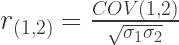
The matrix values I used above are actually designed to generate a pair of variables that are correlated at roughly r = .5. Let’s check out a simplified version of the Pearson’s r formula to see why:

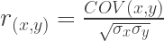
When calculating Pearson’s r (the correlation coefficient), we’re computing a standardized statistic (which is why we are reducing the covariance by expressing it in terms of the standard deviations of the component variables). A couple of basic things to keep in mind here (and in general) include:
- Variances can’t be negative. If you’re trying to simulate data with a negative correlation present, don’t choose negative values for the variances in your matrix code. Variances are based on sums of squared deviations, which means all of the numbers that go into calculating them are positive.
- Covariances can be negative. If you want negative correlations, then you definitely should be specifying negative covariances. I provide an example of a negative correlation a bit further down.
So here we have the following covariance matrix, based on the thing I literally just did like a minute ago:
##      [,1] [,2]
## [1,]    9    6
## [2,]    6   16
Where:
- variance 1 (σ1) = 9 (first element on the diagonal)
- variance 2 (σ2) = 16 (second element on the diagonal)
- covariance (1,2) = 6 (the off diagonals)
Also recall that variances are just squared standard deviations. This also means that standard deviations are just the square roots of variances (and now you’re probably getting why we just happened to set the variances above to two perfect squares. It ain’t a coincidence).
We can slightly change the first formula above to reflect this. That would give us this new, modified formula:

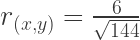
To really make things consistent with our matrix, let’s go even further and change the notation of the variables themselves:
So if we plug in the values from the matrix, we get:

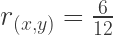
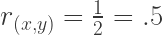
So, the correlation between the two variables is roughly r = .5. I say roughly, because the data are simulated using a multivariate normal random sampling procedure. This process is stochastic (i.e., it unfolds randomly. It can’t be controlled. It can only be given a general set of instructions based on the population parameters that we define for it and feed into it at the start). Because it’s stochastic, it will try hard to produce statistics that are close to what I’m asking for, but it isn’t ever guaranteed to give me exactly what I want. In fact, probabilistically speaking it is entirely possible for a simulation like this one to give me values that are really far off of what I requested (though it is generally unlikely). This kind of random or stochastic weirdness generally becomes less likely as I increase the number of samples (the N value in my initial code) I want the process to conduct before computing its final values. Much like actual random sampling from a population in real research settings, the more observations you simulate from a population, the more likely it is that your simulated sample statistics will resemble the actual population parameters.
We can check what the process gave us with a quick bit of code:
cor(df1)## [,1] [,2]
## [1,] 1.0000000 0.4957285
## [2,] 0.4957285 1.0000000OK, so it gave us r = .50 (I’m rounding here). That’s a damn good job. Though bear in mind, this process is still stochastic, and still capable of going off the rails, even at large sample sizes. In fact, I poked around and found a test case that gave me a dud, despite drawing more values from the population than I originally wanted.
#increasing to 200 doesn't necessarily help.
set.seed(04182019)
df1.with.lame.sauce <- mvrnorm(200, mu=mu, Sigma=sigma)
cor(df1.with.lame.sauce)
## [,1] [,2]
## [1,] 1.0000000 0.4407063
## [2,] 0.4407063 1.0000000We doubled our sample size, and still we got an even worse correlation estimate than we wanted. It’s random, man. The only way to really be confident that the sim will start reliably giving you the values you request is to crank the number of draws way up. Like way, way up. Think like 5,000 and up. I’d say 10,000 as a minimum just to be safe (and if your computer can handle that kind of intensive computation). For example:
#increasing to 10,000 does help though.
set.seed(04182019)
df1.with.extra.turbo.lazer.wolf.sauce <- mvrnorm(10000, mu=mu, Sigma=sigma)
cor(df1.with.extra.turbo.lazer.wolf.sauce)
## [,1] [,2]
## [1,] 1.0000000 0.5027333
## [2,] 0.5027333 1.0000000r = .5027. A solid outcome, if you ask me. Then again… what do we say… 100,000 draws? Hey, why not.
#Now we're just getting ridiculous.
set.seed(04182019)
df1.with.extra.mega.ultra.turbo.lazer.wolf.sauce <- mvrnorm(100000, mu=mu, Sigma=sigma)
cor(df1.with.extra.mega.ultra.turbo.lazer.wolf.sauce)
## [,1] [,2]
## [1,] 1.0000000 0.5003652
## [2,] 0.5003652 1.0000000r = .5004. I like that value as well. Let’s move on.
Setting your own correlation values.
We can rearrange the correlation formula to figure out how to set correlations between two standard normal variables to any value we need (or at least attempt to set it – remember the simulation is stochastic). Here’s how we can fix the value of r to a value we desire:
becomes:

We can set the correlation to a value we want, and fix the variances of the variables to any reasonable values we wish. I say “reasonable” just because it’s usually unnecessary to simulate two correlated variables with wildly different variances, unless you’re trying to simulate data that look this way in reality. If you’re merely testing a data analytic process or conducting sims for teaching purposes, I wouldn’t bother with such a messy setup.
So let’s say we want the correlation between X and Y to be r = -.3 instead. For the sake of ease, we’ll set the variances of V1 and V2 at manageable values of V1 = 9 and V2 = 16 again. We can plug them into the rearranged equation above to find the covariance value we’ll need to specify for our sim population:

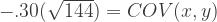
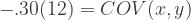
So if we want a correlation of -.3, and we still have variances of 9 and 16, we’ll need a covariance of -3.6 Let’s go ahead with these values for our second sim then:
N2 <-100                           #setting my sample size
mu2 <- c(2,3)                      #setting the means again
sigma2 <- matrix(c(9,-3.6,-3.6,16),2,2)  #setting the covariance matrix values. The "2,2" part defines the number of rows and columns

set.seed(04182019)  #setting the seed value so I can reproduce this exact sim later if need be
df2 <- mvrnorm(n=N2,mu=mu2,Sigma=sigma2)  #simulate the data, as specified above
cor(df2)
## [,1] [,2]
## [1,] 1.0000000 -0.2858137
## [2,] -0.2858137 1.0000000As we see above, our changes yielded a Pearson’s r = .29, which is pretty close. We can use this procedure to create sets of variables to simulate and test all sorts of ideas that call for multivariate data.
Simulating multivariate data with all correlations specified
This one can get complicated pretty quickly, but follows the same logic. For ease, let’s limit it to a system of three variables. Let’s call them X1, X2, and Y. Let’s say that the three correlation values we want are as follows:


If this is what we want, we have to do some quick calculations and decide on variances. Again, lets keep things simple and limit ourselves to just working with perfect squares:
- variance X1 = 16
- variance X2 = 25
- variance Y = 9
We can plug these values into the rearranged covariance equation, one pair at a time, to find the values we need. This gives us the following (note I flipped the order of the terms below, just to make it easier to read):


So we’ll need to set the covariances in the matrix in the R code like so:
| X1 | X2 | Y | |
|---|---|---|---|
| X1 | var X1 = 16 | cov(X2,X1) = 4 | cov(Y,X1) = 4.8 |
| X2 | cov(X1,X2) = 4 | var X2 = 25 | cov(Y,X2) = 9 |
| Y | cov(X1,Y) = 4.8 | cov(X2,Y) = 9 | var Y = 9 |
N3 <-500                           #setting my sample size. let's boost it to accommodate a larger set of variables.
mu3 <- c(6,7,5)                      #setting the means again
#now we're setting the covariance matrix values. This time it's 3x3 so we need to pay closer attention to the order.
#I find it helpful to break it up into an actual matrix, so I don't lose track of which element of the matrix I'm entering:

sigma3 <- matrix(c(16 ,  4,  4.8,
                   4  , 25,    9,
                   4.8,  9,    9),3,3)


set.seed(04182019)  #setting the seed value so I can reproduce this exact sim later if need be
df3 <- mvrnorm(n=N3,mu=mu3,Sigma=sigma3)  #simulate the data, as specified above
cor(df3)
## [,1] [,2] [,3]
## [1,] 1.0000000 0.2374055 0.3918596
## [2,] 0.2374055 1.0000000 0.5801548
## [3,] 0.3918596 0.5801548 1.0000000Recall that we wanted:
and the sim gave us:
So it gave us fairly reasonable approximations of these relationships in a sample of 500 (I increased it to accommodate estimating relationships among a larger system of variables).
We can go on in this fashion to yield what we need. Again, we can crank this sample size up to be more confident that we’ll get estimates that are more akin to what we’ve told the simulation about the actual population values.
That pretty much does it. Go have fun. Me? I’m going to sleep.


Lifesaver!